Transformers: The AI Revolution Behind ChatGPT & Other LLMs!

Understanding Machine Learning Series

Introduction to Transformers - the building blocks of Large Language Models

Motivation

The release of ChatGPT by OpenAI in Nov. 2022 is a pivotal moment in the era of AI-driven systems, not only from a technical standpoint, but also in gaining widespread popularity beyond the machine learning research community. It would not be an exaggeration to say that ChatGPT revolutionized the way in which non-technical people interact with AI-systems in their everyday life. Though the general public might be in awe about some conversational-AI model and be content with its functionalities, we, tech-savvy people, would like to deconstruct such a complex system in order to understand its inner workings.

So, where shall we begin? First and foremost, ChatGPT belongs to a family of Large Language Models (LLMs) called Generatively Pre-trained Transformers (GPTs) and is designed to generate human-like responses in a wide range of contexts. The Transformer model, in its turn, uses the mechanism of (self-)attention (don't worry, the remainder of the article is all about understanding this!) to process and understand relationships within sequences of text, thereby enabling the system to generate coherent and contextually relevant responses.

In this article, we will be focusing on understanding the mechanism of attention as originally introduced in the context of Machine Translation models in Natural Language Processing (NLP). Let's get started!

1.What is machine translation ?

In NLP, Machine Translation is the task of using computational techniques to translate text from one language (called the source language) to another language (called the target language). For example,

Input: It is not what you say, but how you say it. (English)

Output: C'est le ton qui fait la chanson. (French)

We can clearly see two things here: (i) the number of words in the input and output sentences are different and (ii) a word-to-word mapping from one language to another using some kind of a lookup-table would be useless (for all practical purposes)! In fact, the words in the output French sentence le ton which means the tone / the sound and la chanson meaning the song don't even appear in the input English sentence.

Now, the question arises: how are we going to achieve this?

2.Sequence-to-Sequence (Seq2Seq) Models

Let us go back in time, to 2014, the period when Convolutional Neural Networks (CNNs) have impressed the world by their extraordinary capabilities in classifying images. At the same time, Recurrent Neural Networks (RNNs) were the most popular choice of architecture for processing sequential data such as text. Some different kinds of tasks that can be accomplished using RNNs can be seen below:

a. Seq2Seq with RNNs

One straightforward way to accomplish the task of MT is to use a simple RNN-based Sequence-toSequence model. It consists of two networks connected in a cascaded fashion:

i) An input encoder: Encodes the input sequence into a single vector, called the context vector

ii) An output decoder: Produces the output sequence from the single context vector

Mathematically, given an input sequence x₁, …, x_T , the encoder computes the sequence of hidden states in a recurrent manner as follows:

h_t = f_W(x_t, h_t-1),    for t = 1,...,T     (2.1)

Taking the final hidden state h_T and setting it as the context vector c, the decoder computes its hidden states as

s_t = g_U(y_t-1, s_t-1, c)    for t = 1,...,T'     (2.2)

and the output tokens are sampled according to y_t ~ σ(U_yss_t).In eqns. (2.1) and (2.2), f and g represent the encoder and decoder RNN networks with their shared weight matrices W and U respectively. Here, y₀ is set to [START], a special token that marks the beginning of a sentence and the sampling process goes on till T' when y_T' = [STOP] gets sampled. The following animation depicts a Seq2Seq model which translates an English sentence into Spanish.

For more details on how the network is trained including some architectural tweaks which guarantee good results, you can refer to Sutskever et al.. There is a serious drawback in the above architecture: the input sequence is bottlenecked through a single vector (of fixed size), i.e. the context vector is supposed to capture the essence of the entire input sequence. This does not work well, especially when the input sequences (i.e. sentences in the source language) are very long. To overcome this issue, Bahdanau et al. propose the idea of using a new context vector at each step of the decoder. i.e. they propose an extended version of the above model where they allow the model to automatically select parts of the input sentence that are relevant to predicting a target word.

b. Seq2Seq with RNNs + Attention

Rather than attempting to encode the input sequence into a single vector, this model encodes the input sequence into a sequence of vectors. At every timestep of the decoder, some subset of these vectors are adaptively used to predict the target word. Thus, this model learns to align and translate jointly.

As in the previous model, the encoder computes a sequence of hidden states in a recurrent manner. The initial state of the decoder s₀ is set to h_T. Then, we can compute:

• The scalar alignment scores e_t,i = f_att(s_t-1, h_i) for all encoder hidden states h_i's at every timestep t of the decoder. Here, f_att is an alignment model, which can be a simple MLP that measures how much inputs around position i are relevant to decoding the target word at position t.
• Then, these raw scores are normalized to produce the attention weights

  0 < a_t,i < 1 and ∑_ia_t,i = 1       (2.3)

  The above attention weights can be computed using a softmax activation layer.
• Then, the context vector for decoder at timestep t is computed as a weighted sum of the encoder hidden states   h₁, ..., h_T using

  c_t = ∑_i a_t,ih_i    (2.4)

• Finally, the decoder hidden states are computed using

  s_t = g_U(y_t-1, s_t-1, c_t)     for t = 1,...,T'   (2.5)

  
  The output tokens are sampled in a similar way as described above. The above computations can be visualized as follows:

Clearly, all the operations introduced above are differentiable. Hence, there is no need to supervise the attention weights - backpropagation will work its magic as usual!
Using a different context vector at each timestep of the decoder gives us two main advantages:

• Input sequence's representation is no longer bottlenecked through a single context vector
• At every timestep, the context vector 'looks at' / 'attends to' the relevant parts of the input sequence

The second point above can be exemplified with the following example. Consider an English to French translation task where the input 'The agreement on the European Economic Area was signed in August 1992.'' is translated as ''L'accord sur la zone économique européenne a été signé en août 1992.''. Visualizing the attention weights shows that the model has indeed learned to align while translating the sentence: in the animation below, black represents the value 0 and white represent 1, while shades of gray represent the values in-between.

If we observe eqn 2.4. closely, we can see that, at every timestep, the decoder does not take into account the fact that h_is form an ordered sequence! It just treats them as an unordered collection, or equivalently, a set of vectors. This motivated researchers to use this architecture even for non-sequential data like images for tasks such as image captioning. The images are first passed through a CNN backbone to extract a grid of features. The grid is subsequently divided into blocks which play a role analogous to the hidden states in the encoder. For more details on how the mechanism above can be used for image captioning, read this excellent work by Xu et al.

3.The Attention Mechanism

The research community realized that the concept of attention used in the above models is fundamentally different from other kinds of layers known to them (fully-connected/ convolutional/ recurrent layers). Naturally, they wanted to create a new general-purpose layer out of it, which can be used in a variety of contexts.

Let us now formulate what is known as the Scaled Dot Product Attention (SDPA) used widely today in most of the LLMs (of course, with slight modifications needed for improvement). Instead of directly dropping the final expressions, let us try to build it in an intuitive manner.

Stage 1: Let q ∈ ℝ^D_q be the query vector and X ∈ ℝ^{N_x × D_q} be the set of inputs. Using scaled dot product as a similarity measure, the vector of similarities e can be computed as:

e_i = (q · X_i)/√D_q    i = 1, ..., N_x    (3.1)

Now, there are two things to be understood:

i) to understand the scaling factor of 1 / √D_q : without loss of generality, assume q_is and the entries of X_is are all independently and identically distributed random variables with mean 0 and variance 1. Then, the dot product between these vectors will have a variance D_q. So, in order to keep the variance of the dot product equals to 1, we scale it appropriately.
ii) More importantly, why do we need to keep the variance as unity? The reason is that these similarities will be subsequently subjected to go through a softmax layer. With large values, the similarities will saturate the softmax layer leading to vanishing gradients problem.

Then, the attention weights a ∈ ℝ^N_x could be computed as

a = softmax(e)    (3.2)

Finally, the output vector is computed as a linear combination of the inputs where the weights are the attention weights computed in (3.2) using

y = ∑_i a_iX_i    (3.3)

Stage 2: Let us now generalize this even further. Assume that we have N_q query vectors arranged in a matrix Q ∈ ℝ^{N_q × D_q}. We can now compute a matrix of similarities E ∈ ℝ^{N_q × N_x} whose entries are given by:

e_i,j = (Q_i · X_j)/√D_q    i = 1, ..., N_q and j = 1, ..., N_x   (3.4)

Here, the matrix of attention weights A ∈ ℝ^{N_q × N_x} is computed by

A = softmax(E, dim=1)   (3.5)

Clearly, row i of A is a probability distribution which gives the similarity between query Q_i and all other inputs. So, we can compute the outputs Y ∈ ℝ^{N_q × D_q} using

Y = AX    (3.6)

Stage 3: Now, we are ready to formulate the mechanism of self-attention as it is used in transformers.. We need to make the following transformations:
(i) Instead of using the inputs directly, we produce key vectors K and value vectors V that are obtained by simple learnable linear projections of the inputs X.
(These terminologies of queries, keys and vectors are adapted from the literature of Information Retrieval (IR) systems. To understand these terms with a simple analogy, imagine we are searching for something on Google search. The text we enter into the search bar constitutes the query. The search engine will then match our query to the indexed-terms (play the role of keys) in its database. Based on this matching process, relevant documents (values) are returned to the user finally.)
(ii) Instead of having an arbitrary number of queries, we will compute one query per input vector using a suitable projection matrix.
The various quantities involved and the computations happening are summarized in the tables below:

Inputs
Input vectors: X (shape: Nx × Dx)
Query projection matrix: Wq (shape: Dx × Dq)
Key projection matrix: Wk (shape: Dx × Dq)
Value projection matrix: Wv (shape: Dx × Dv)

Computations
Query matrix: Q = XWq
Key matrix: K = XWk
Value matrix: V = XWv
Similarities: E = QKT (shape: Nx × Nx)
Attention weights: A = softmax(E, dim = 1) (shape: Nx × Nx)
Outputs: Y = AV (shape: Nx × Dv)

The above computations can be pictorially represented as:

Here,W_q, W_k and W_v are all learnable parameters and they are learnt through backpropagation.
Permutation equivariance: The architecture that we show above has an interesting property. Consider permuting the input vectors. What do you think will happen to the outputs then? Let's try to visualize this.

Clearly, the queries and the keys computed are the same but in the permuted order. Consequently, similarities and attention weights are also the same as before with the only difference being they are in the permuted order. Also, the values which also follow the same permuted order result in the same set of outputs as before but in the permuted order. This entire process can be elegantly summarized in the following equation. If the entire network above can be represented as some differentiable operator f, then any permutation o(.) applied on the inputs x simply translates to permuting the outputs of the network, i.e.

f(o(x)) = o(f(x))    (3.7)

This property is known as the permutation equivariance nature of the self-attention layer. It is clear that the self-attention layer, as formulated above, doesn't know the order of the vectors it is processing. So, for practical use with text sequences in which words appear in order (note that order is essential to retain the meaning of the sentence), we need to concatenate the input vectors with positional encoding. (Positional encodings deserve an article of their own! So, more on this in a future blog!)

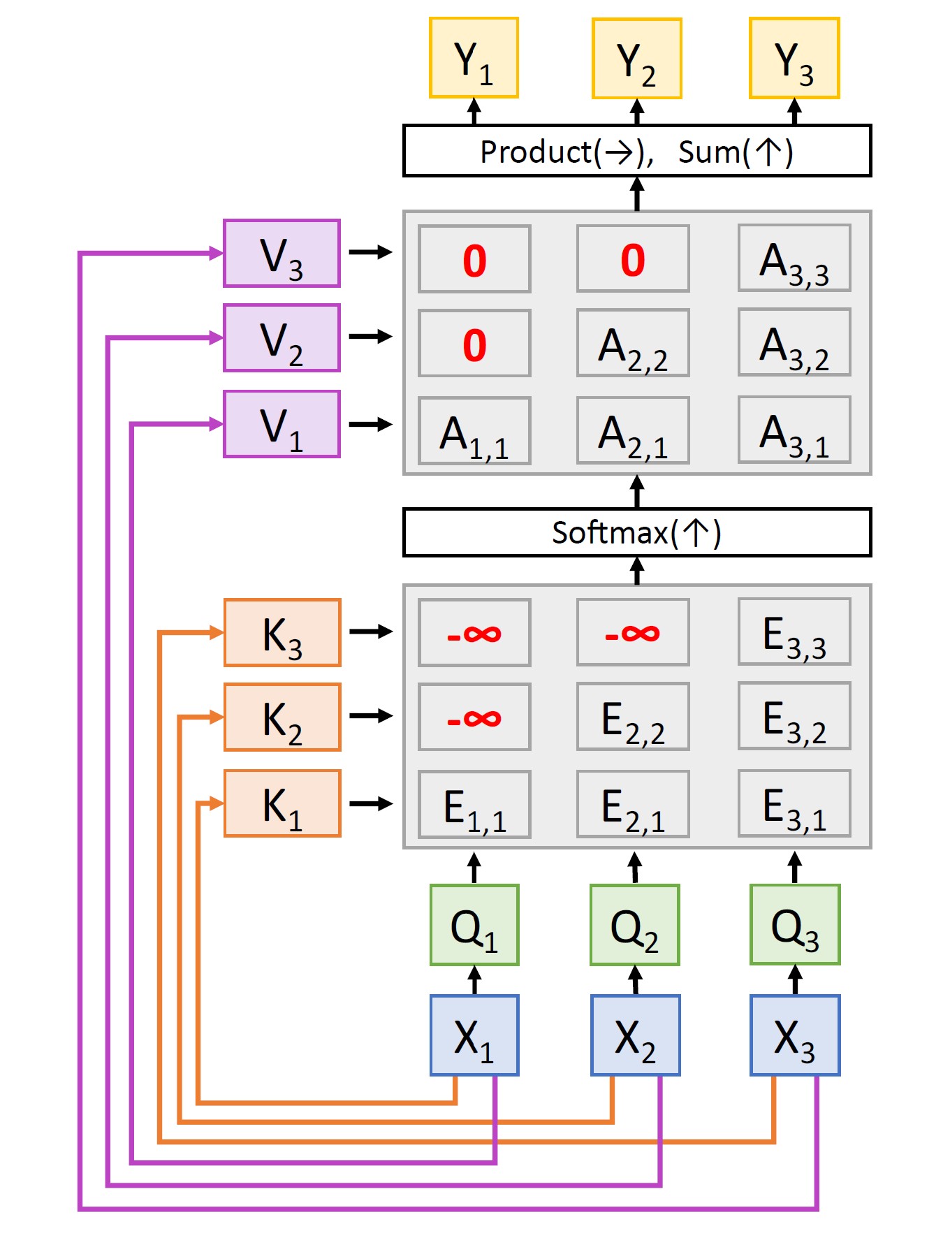
Masked Self-Attention Layer: This is a slight variation on the above architecture wherein we do not allow the model ''to look ahead'' or ''to look into the future.'' This is useful in Language Modelling (LM) tasks where the network has to predict the next token based only on the tokens seen so far. This can be easily achieved by setting the similarities corresponding to future vectors to −∞. That way, when softmax is applied, the attention weights turn out to be 0.

Multihead Self-Attention: Instead of using one set of QKV projections, multi-head attention splits the input into multiple sets of QKV projections using multiple attention heads that run in parallel (wherein each head has its own set of projection matrices W_q^h, W_k^h, and W_v^h, where h = 1, …, H is the index into the number of attention heads). Thus, inputs are projected onto different subspaces using head-specific learnable weight matrices. Each of the heads independently computes its SDPA in parallel. To maintain computational complexity, each of the individual heads works at a much lower dimension. Finally, the output from all the heads is concatenated and linearly transformed using yet another learnable projection matrix W_o to produce the final output.

There are two main advantages of using a multihead attention layer: (i) Using multiple heads enriches the learning capabilities of the attention layer, wherein each head can learn to model different relationships between input tokens. For instance, one head could focus on learning syntactic structure, another could focus on learning the underlying semantics, whereas another head could focus on modeling long-range dependencies. (ii) The resulting architecture is highly scalable and efficient (since all the heads' outputs can be computed in parallel).

4.The Transformer block & The Transformer

Here we are! We now have all the pieces required to build the transformer block as introduced in the work from the Google Brain Team in 2017 (one of the most cited papers in the entire deep learning literature). The transformer block introduced by Vaswani et al. uses stacked self-attention and point-wise Feed-Forward (FF) network (2 fully-connected (FC) layers with a ReLU activation in between) for both the encoder & the decoder as shown below:.

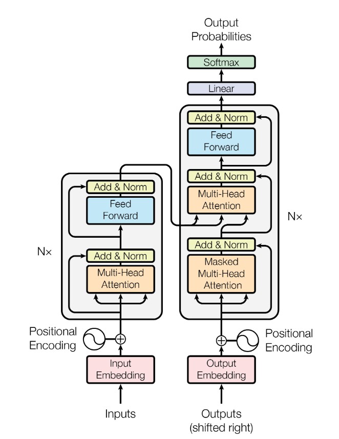
Clearly, the Transformer block follows the overall architecture of Seq2Seq model with an encoder-decoder architecture.

Encoder stack: The encoder consists of N=6 identical layers stacked on top of each other. Each of the layer has two sub-layers. The output of each of the sublayer is of the form LayerNorm(x + Sublayer(x)), where Sublayer is one of Multihead Self-Attention layer or a simple FC Feed-Forward network. To facilitate addition of residual layers' outputs, all the sublayers (including the embedding layers) produce outputs of dimensions 512.

Decoder stack: The decoder is also a stack of N=6 identical layers. In addition to the two sublayers in the encoder, we here have a third sublayer that performs multihead attention over the output of the encoder stack. Also, we can see the use of Masked multihead attention layer in the decoder to prevent the model from attending to subsequent tokens. Along with shifting the output embeddings by one position, this masking makes sure that predictions for a given token depends only on the previous tokens that have been generated so far.

A closer observation reveals that the transformer block uses multihead attention in three different ways:

• The self-attention layers in the encoder get their queries, keys, and values from the same place—the output of the previous layer in the encoder. So, each position can attend to all other positions in the previous layer of the encoder.
• Similarly, in the decoder, the self-attention layers allow every position to attend to all positions up to and including that position (due to the masking), thereby preventing looking ahead in the sequence. Technically, this makes the decoder auto-regressive in nature.
• Those attention layers that are at the transition point between the encoder and decoder have queries coming from the previous decoder layer, whereas the keys and values come from the output of the encoder. This allows every position in the decoder to attend over all positions in the input sequence (as is the case in the Seq2Seq models we discussed previously!).

Due to the numerous advantages of the multihead architecture listed in the previous section, the authors propose a transformer block that uses multihead attention with H = 8 heads. As discussed above, to keep the computational complexity constant, each of these heads works with 512 / 8 = 64 dimensions.

Yet another thing to notice is that the self-attention module is the only place where there is interaction between the vectors, whereas both the LayerNorm and the FC FF-network act independently on each vector. For more details on the kind of positional encodings used and a comparison of computational complexities of different kinds of layers (such as convolutional, recurrent, and attention layers), please read the manuscript cited above.

5.Conclusion

In this article, I have tried to explain the Transformer architecture as a natural solution for addressing the problem of machine translation. But that is not all it can do! Would you like to know how the transformer is used to build LLMs like BERT, GPT or T5? Stay tuned!

References

- Most of the animations / images were adapted from Prof. Justin Johnson's lecture notes here.
- To learn more about LayerNorm, please consult the paper by Jimmy Ba et al here.
- 3Blue1Brown's video on Transformers with amazing visualizations as usual can be found here.
- In this article, I have used a bottom-up approach in building the Transformer block. If you want a complementary top-down approach of breaking it down, read this excellent blog entitled The Illustrated Transformer by Jay Alammar.